CS 486/686 Lecture 2 — Uninformed Search

CS 486/686
Uninformed Search

Yuntian Deng

Lecture 2

RN 3.1–3.4

Learning goals

Formulate problems as search
Trace DFS, BFS, IDS
Analyze: space, time, completeness, optimality
Pick the right algorithm

Heads-up: Chat 1 is live

Use your WatIAM @uwaterloo.ca email (not your friendly one)
Verify the email Chrysalis sends; you'll be auto-added to CS 486/686
Chat 1 covers L1 + L2 — due Tue May 26, 11:59 PM (one-time extension for late enrollees)
Issues? Private Piazza post to Prashanth Arun & Robert Cai (Chrysalis designers)

Full instructions: course page → Chat Assignments with Chrysalis.

Where does search show up?

Robotics

Route planning

TSP

        \( ((a \land b) \lor c) \land d \)
        
\( \lor (\neg e) \)

SAT

8-puzzle

River crossing

N-queens

…

And many more

TSP: Quanta. SAT / FCC auction: UBC news.

Why search?

Sequential decisions
No closed-form algorithm
Easy to verify, hard to find
Systematic, not guesswork

What is a search problem?

Five components:

States
Initial state
Goal test
Successor function
Cost (optional)

Solution = path from start to goal.

State spaces are huge

1.8 × 10⁵

8-puzzle

3×3 sliding tile

10¹³

15-puzzle

4×4 sliding tile

4.3 × 10¹⁹

Rubik's cube

3×3×3

Too many states to enumerate. We need clever search.

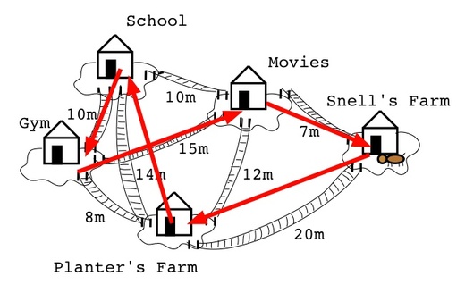
Search graph

States → nodes
Actions → edges
Goal: find a path S → G

Search tree & frontier

Don't enumerate the graph
Grow a tree from S, one path at a time
Frontier = paths to expand next

Example: 8-puzzle

Initial

Goal

State: 9 positions, 0 = empty
Initial: 530,876,241
Goal: 123,456,780
Successor: slide adjacent tile into empty
Cost: 1 per move

181,440 reachable states — too many to enumerate.

Quick check: successors

Q. Which is a successor of 530,876,241?

350,876,241
536,870,241
537,806,241
538,076,241

Initial

B. Slide the 6 up.

Multiple formulations possible

State def → nodes
Successor → edges
Minimize both

Same 8-puzzle, different state

By grid

9 cells, 0–8

By coordinates

        \((x_0, y_0), (x_1, y_1),\)

        \((x_2, y_2), \ldots, (x_8, y_8)\)
      
9 (x,y) pairs — ~2× the space

Successor swaps empty tile's coords with a neighbour's.

Generic search algorithm

// Inputs: graph, start node s, goal test goal(n)
function Search(graph, s, goal):
    frontier ← { <s> }
    while frontier is not empty:
        select and remove a path <n₀, …, n_k> from frontier
        if goal(n_k):
            return <n₀, …, n_k>
        for each neighbour n of n_k:
            add <n₀, …, n_k, n> to frontier
    return “no solution”

expand: pop path → get neighbours → push extended paths

One template, three algorithms

DFS, BFS, IDS all use this skeleton.

They differ only in which path they pull from the frontier.

Depth-first search (DFS)

Frontier = stack (LIFO)
Pop newest
Dive deep, then backtrack

Trace: DFS

Push children alphabetically. Step numbers = order of expansion.

Frontier: (S) (D, E, P) (D, E, Q) (D, E) (D, H, R) (D, H, F) (D, H, C, G) goal G reached!

Evaluating search algorithms

Four questions we'll ask about every algorithm:

Space — how much memory? (worst-case frontier size)
Time — how many nodes does it visit? (worst case)
Complete? — is it guaranteed to find a goal if one exists?
Optimal? — does it return the cheapest (or shallowest) goal?

Tree parameters: \(b\), \(m\), \(d\)

\(b\) — branching factor

\(d\) — depth of shallowest goal

\(m\) — max depth of tree

DFS — properties

Space	\(O(bm)\) linear
Time	\(O(b^m)\) exponential
Complete?	No
Optimal?	No

DFS fails on cycles

\(H \to I \to J \to H\) traps DFS forever.

Fix: cycle pruning

Keep a visited set. Skip states we've already expanded.

Order: S → H → I → J → back to H? skip! → G.

DFS takes the first goal, not the best

Returns the long path; ignores the shorter \(S \to D \dashrightarrow G\).

When to use DFS

Good fit

Memory limited
Many goals exist
Deep solutions

Bad fit

Cycles
Shallow solutions
Need optimality

Breadth-first search (BFS)

Frontier = queue (FIFO)
Pop oldest
Level by level

Trace: BFS

Pop the oldest path. Step number = order of expansion. Multiple paths to P and B.

Frontier: (S) pop S → push D, E, P → (D, E, P) pop D → push B, C → (E, P, B, C) pop E → push H, J → (P, B, C, H, J) pop P → push Q → (B, C, H, J, Q) pop B → push P → (C, H, J, Q, P) pop C, H, J (leaves) → (Q, P) pop Q → push B, G → (P, B, G) pop P, B → push Q, P → (G, Q, P) pop G — goal!

BFS — properties

Space	\(O(b^d)\) exponential
Time	\(O(b^d)\) exponential
Complete?	Yes
Optimal?	Shallowest goal (optimal at equal cost)

When to use BFS

Good fit

Memory plentiful
Want fewest arcs
Cycles possible

Bad fit

Deep solutions
Large branching
Graph generated on the fly

What if edges have different costs?

S→A→G: cost 11. S→B→G: cost 6.
BFS picks the wrong one (it's fewer hops, but pricier).

Uniform-cost search (UCS)

Frontier = priority queue
Key = path cost so far
Pop the cheapest path first

Complete + optimal when all costs are positive.

When every edge has cost 1, UCS = BFS. (We'll use BFS in this lecture for that reason.)

BFS vs DFS — Q1

Q. Memory is very limited.

BFS
DFS
Both are fine
Neither

B — DFS. DFS: \(O(bm)\) vs BFS: \(O(b^d)\).

BFS vs DFS — Q2

Q. All solutions are deep in the search tree.

BFS
DFS
Both are fine
Neither

B — DFS. Dives down long paths instead of enumerating every shallower level.

BFS vs DFS — Q3

Q. The graph contains cycles.

BFS
DFS
Both are fine
Neither

A — BFS. DFS can fail to find the goal (gets stuck going deeper into the cycle); BFS still finds any goal at finite depth. (BFS does waste work without cycle pruning — but it's complete.)

BFS vs DFS — Q4

Q. The branching factor is huge or infinite.

BFS
DFS
Both are fine
Neither

B — DFS. BFS's frontier blows up with \(b\); DFS stays linear.

BFS vs DFS — Q5

Q. You must find the shallowest goal.

BFS
DFS
Both are fine
Neither

A — BFS. BFS guarantees the shallowest goal.

BFS vs DFS — Q6

Q. All solutions are very shallow.

BFS
DFS
Both are fine
Neither

A — BFS. Checks shallow neighbours before diving deep.

BFS vs DFS tradeoff

	BFS	DFS
Space	\(O(b^d)\)	\(O(bm)\)
Complete?	Yes	No

Can we have both?

Why \(O(b^d)\) matters

Branching factor \(b = 10\), 1 state = 8 bytes, computer doing 10⁹ states/sec.

Depth \(d\)	States \(b^d\)	BFS memory	Wall-clock time
4	10⁴	80 KB	10 µs
8	10⁸	800 MB	0.1 s
12	10¹²	8 TB	~17 min
16	10¹⁶	80 PB	~4 months
20	10²⁰	800 EB	~3000 years

Doubling \(d\) doesn't make the problem twice as hard. It makes it 10,000× harder.

Iterative-Deepening Search (IDS)

For \(\ell = 1, 2, 3, \ldots\), run DFS up to depth \(\ell\).

Stop when a goal is found.

Each iteration is depth-limited search (DLS).

Trace: IDS

Same graph as BFS. Each iteration is depth-limited DFS.

Depth limit: 1 — visit S only. 2 — visit S, P, E, D (DFS, alphabetical push order). 3 — explore level 3, no goal yet. 4 — S → P → Q → G. Goal found!

IDS — properties

Space	\(O(bd)\) linear
Time	\(O(b^d)\) exponential
Complete?	Yes
Optimal?	Shallowest goal

Summary: DFS vs BFS vs IDS

	DFS	BFS	IDS
Frontier	Stack (LIFO)	Queue (FIFO)	Stack, repeated at deeper limits
Space	\(O(bm)\)	\(O(b^d)\)	\(O(bd)\)
Time	\(O(b^m)\)	\(O(b^d)\)	\(O(b^d)\)
Complete?	No	Yes	Yes
Optimal?	No	Shallowest goal	Shallowest goal

\(b\) = branching factor; \(m\) = max depth of the search tree; \(d\) = depth of the shallowest goal.

DFS vs BFS: exploration order

DFS — dives deep first

BFS — expands by level

Animations by Mre, Wikimedia Commons (CC BY-SA 3.0).

Learning goals (recap)

✓ Formulate problems as search
✓ Trace DFS, BFS, IDS
✓ Analyze: space, time, completeness, optimality
✓ Pick the right algorithm

Next lecture: informed search (heuristics, A*).

Next: informed search

Use a heuristic \(h(n)\) — an estimate of distance to the goal — to bias the search.

A* combines path cost so far (\(g(n)\)) with heuristic (\(h(n)\)) — provably optimal under mild conditions.