From fixed features to learned vector representations
Recorded lecture (asynchronous)
🎥 This lecture is pre-recorded - I'm away at ICML this week, so there's no in-person class today. Watch at your own pace.
📅 Due today (Thu Jul 9): CS686 project proposal. Assignment 2 is now due Thu Jul 16.
💬 Questions? Post on Piazza - the TAs are available, and I'll follow up when I'm back.
What you should take away
One thread runs through the whole lecture: useful vectors can be learned.
build
Explain why hidden layers need nonlinearities.
represent
Explain embeddings as learned vectors, including contextual ones.
inspect
Use projection, neighbors, and clusters to reason about embedding spaces.
The later examples are applications of the same idea: learned spaces become interfaces.
Act 1: learn the features
L17 trained models on fixed input vectors.
Today, the model also learns the vector representation.
The problem with fixed features
L17 assumed the useful input vector already exists.
pixels
Where is the cat ear?
word IDs
Why is dog close to puppy?
screenshots
Which region is a button?
Modern ML learns the features too.
Neural nets learn representations
The hidden layer is not just computation: it is a learned view of the input.
A neuron is a feature detector
inputs \(x_1, x_2, x_3\)
weighted sum: \(z = w^\top x + b\)
activation: \(a = g(z)\)
A real learned neuron
Each character is colored by one neuron's activation in a character-level RNN.
Nobody programmed it — this neuron learned to fire inside URLs.
Karpathy, "The Unreasonable Effectiveness of Recurrent Neural Networks," 2015.
Why add a nonlinearity?
Two linear layers in a row collapse into one:
\(W_2(W_1x)\)\(\,= (W_2W_1)\,x\)
Depth alone adds nothing — we need a nonlinearity between the layers.
The fix: a nonlinearity
Insert \(g\) between layers: \(h = g(W_1x),\quad \hat y = W_2 h\).
\(g(x)=\max(0,x)\)
The bend is what lets stacked layers represent nonlinear functions.
Playground: does nonlinearity matter?live
Same net, activation off vs. on — try it on the live slides.
Interactive on the live slides: the same 1-hidden-layer net trains to fit a wavy target. With the activation OFF it can only draw a straight line; turn it ON and the layer bends to follow the curve.
One hidden layer = learned feature map
Each hidden unit learns a detector.
The output layer combines detectors.
This is how fixed features become learned features.
XOR: why hidden features help
A hidden layer can transform the space.
Then a simple output layer can solve the task.
Playground: train a net on XORlive
Train a tiny net on XOR — try it on the live slides.
Interactive on the live slides: a tiny 2-2-1 network trains on XOR with real forward passes and backprop. Watch the decision surface bend and the loss drop until the two classes separate — something no straight line can do.
An MLP: a bigger model, same loop
\(h = g(W_1x+b_1)\)
\(\hat y = \mathrm{softmax}(W_2h+b_2)\)
Every operation is differentiable, so L17's training loop applies unchanged.
Quick check: what changed from logistic regression? Only the function class, not the optimization recipe.
The code barely changes
model = nn.Sequential(
    nn.Linear(d_in, 64),
    nn.ReLU(),
    nn.Linear(64, n_classes),
)

loss = loss_fn(model(x), y)
loss.backward()
optimizer.step()
The function is richer; the training pattern is the same.
Backpropagation assigns credit
Mechanically, this is the chain rule applied through the computation graph.
What do hidden layers learn?
Deep models compose simple features into useful abstractions.
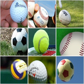
CNNs learn visual features
shallow: curves→middle: parts→deep: objects
one deep neuron = a "ball" detector
Feature visualizations (what each neuron responds to most). Olah et al., "Feature Visualization," Distill 2017 (CC-BY).
Local filters detect small patterns.
Shallow: edges & curves.
Deeper: object parts.
Deepest: whole objects.
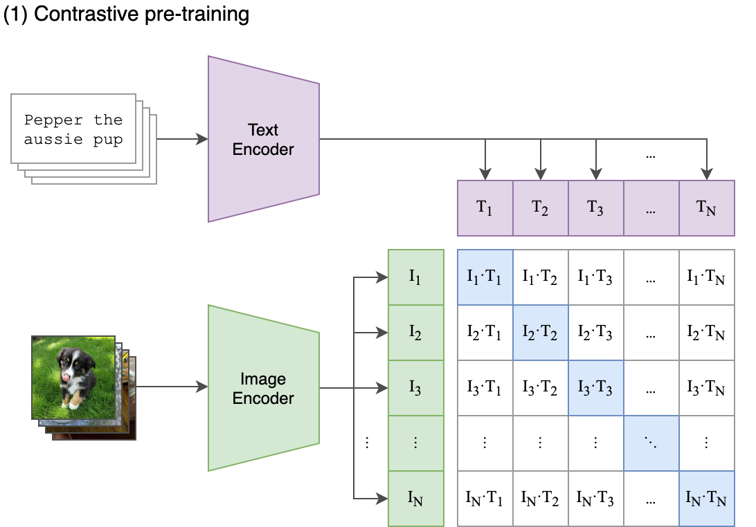
Later: VLMs reuse image encoders (L23).
Act 2: embeddings give symbols geometry
The same representation idea applies when the input is not pixels, but tokens.
A word ID is just a label; an embedding is a learned location in a vector space.
Word IDs have no geometry
IDs are arbitrary labels:
cat = 17, the = 18, dog = 932
id 17 (cat) is no closer to id 18 (the) than to id 932 (dog) — adjacency means nothing.
An embedding gives each a vector, where distance = similarity:
Similar meaning → nearby vectors (cat close to dog; "the" is off on its own).
An embedding table is a learnable lookup
It is just a lookup table (a dictionary): a token's id selects its row.
Unlike a fixed dictionary, the rows are parameters: gradient descent updates them during training.
How does an embedding learn?
Words in the same contexts get pulled together: I have a ___ cat is usually a color.
brown
black
white
To fill the same blanks, the model gives these color words similar embeddings.
Directions can carry meaning
king − man + woman ≈ queen
Add the "royal" direction to man and you land near woman (word2vec, GloVe).
Today this is learned implicitly inside LLMs; contextual vectors rarely do clean arithmetic.
One word can mean two things
"I ate an apple" → fruit
"Apple released a phone" → company
A single fixed vector for "apple" cannot be both.
Modern models embed the whole sentence, so a word gets a different contextual vector each time.
This creates the L19 problem: context has to move information between token vectors.
Act 3: inspect learned spaces
Once inputs become vectors, we can ask geometric questions.
project
Can I see the space?
neighbors
What is close to what?
cluster
What groups exist?
Inspect embeddings by projecting themlive
PCA keeps the directions of most spread — drag the cloud, then flatten it.
Interactive on the live slides: rotate a real 3D point cloud and watch PCA flatten it onto the 2D plane that captures the most variance (the thin 3rd direction is dropped). PCA is linear; t-SNE/UMAP are nonlinear alternatives.
PCA on real data: a million chatslive data
Real WildChat conversations (1536-dim) projected to 2D — hover to read, click to open.
Interactive on the live slides: each dot is a real conversation, embedded to 1536 dimensions with OpenAI's text-embedding-3-small and projected to 2D with PCA. Hover a dot to read its first message; click to open the full conversation. From WildVis (Deng et al.), wildvisualizer.com.
Playground: embed real wordslive model
Type words or sentences; a real model embeds them — try it on the live slides.
Interactive on the live slides: type any words or short sentences and a real embedding model (MiniLM, via Transformers.js) turns each into a vector; PCA projects them to 2D and you click a point to see its nearest neighbors. Dog lands near puppy, car near truck, king near queen — geometry the model learned from data.
Cluster embeddings with k-means
After embeddings exist, k-means becomes a way to summarize the space with prototypes.
inspect datasets
find groups or duplicates
build codebook intuition: replace many vectors with a few representative centers
The k-means algorithm
1. Choose \(k\); initialize \(k\) centroids (e.g. random data points).
2. Repeat until assignments stop changing:
a. Assign — put each point with its nearest centroid.
b. Update — move each centroid to the mean of its points.
Converges to a local optimum — depends on initialization, so run a few times and keep the best.
Playground: k-means, step by steplive
Step through assign and update — try it on the live slides.
Interactive on the live slides: press Step to run one round of Lloyd's algorithm — assign each point to its nearest centroid, then move each centroid to the mean of its members. Repeat until the clusters stop changing. Reseed for a fresh layout.
Act 4: learned spaces become interfaces
So far, we used embeddings for individual points, neighbors, and clusters.
Next: use learned spaces to compare distributions, compress data, and align modalities.
How do you grade an image generator?
Prompt "a dog" — every sample is a different valid dog.
dog A
fluffy, sitting
dog B
running, brown
dog C
puppy, close-up
There is no single ground-truth image to compare against.
So compare the whole distribution of outputs to real images.
Measuring image quality: FID
Embed real and generated images with an Inception network, then compare the two distributions in feature space.
FID = distance between the two feature distributions — lower means the generations look more real.
Heusel et al. 2017.
How do you grade a story generator?
Ask for a short story — there are countless good ones.
story A
a lost dog finds home
story B
a robot learns to paint
story C
two friends and a map
No ground-truth story to score against.
So compare machine stories to human stories as distributions.
Measuring text quality: MAUVE
Embed human and machine text in a language model's space and compare the two distributions.
MAUVE summarizes how much the two distributions overlap — higher means more human-like.
Pillutla et al. 2021.
Autoencoders learn compression
Another use of learned spaces: store what matters in a smaller latent vector.
Latent diffusion will generate in a compressed latent space.
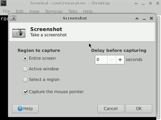
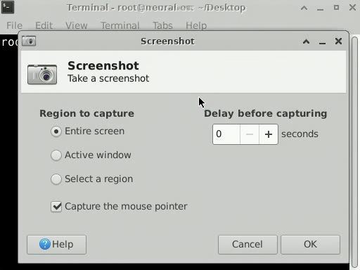
A real autoencoder: NeuralOS
input→
encoder
→
latent z→
decoder
→reconstruction
The decode looks the same as the input — the small latent kept everything that matters.
This makes the latent a useful interface: compact enough to model, rich enough to reconstruct.